Compiled Notes for Microeconomics
Most of the content and all images used are from the book “Principles of Economics” by Gregory Mankiw.
- Lecture 1
- Lecture 2
- Lecture 3
- Lecture 4
- Lecture 5
- Lecture 6
- Lecture 7
- Lecture 8
- Lecture 9
- Lecture 10
- Lecture 11
- Lecture 12
- Lecture 13
- Lecture 14
- Lecture 15
- Lecture 16
- Lecture 17
Lecture 1
Economics is the study of how society manages its scarce resources.
-
There is no such thing as a free lunch. The common trade-off is between efficiency (society is making the best of the scarce resources) and equality (benefits are distributed equally).
-
The opportunity cost of an item is what we give up to get something - the greatest cost in going to college is not money, but time, which is an opportunity cost.
-
Economists assume that people are rational and look at things marginally - the changes that occur when we make a small change to our plan of action. Rational people make decisions by looking at marginal benefits and costs.
-
People respond to incentives. When policymakers fail to consider how their policies affect incentives, there are often unintended consequences. Example: see page 8 (seatbelt law)
-
Trade can make everyone better off. People gain from their ability to trade and competition results in gains from trading. Trade allows people to specialize in what they want. There is something called the Robinson Crusoe economy wherein there is no possibility of trade (Robinson Crusoe was the only person on the island so he had to produce all the goods for all his needs). This is a protectionist approach and tries to make the units completely self-reliant. On the other hand, liberalism asks people to focus on their strengths and encourages trade.
-
Markets are (usually) a good way to organize economic activity. A market economy allocates resources through the decentralized decisions of many firms as they interact in markets. It is a decentralist approach. Households/firms separately decide who/what to hire/work for/buy/produce. Adam Smith observed that households/firms act as if they are guided by an “invisible hand”. Althought they act separately, the system doesn’t crash. This invisible hand is just supply and demand and prices are the instrument using which 「the hand」 directs market activity. Because households/firms look at prices when they make decisions, they unkowingly account for the social costs of their actions. Individual supply and demands get converted to social supply and demands, which results in the aggregating of individual entities. This results in decision makers reaching outcomes that maximise the welfare of society. When this invisible hand is disrupted (perhaps by the government), there can be adverse affects such as how taxes adversely affect resource allocation.
-
Governments can improve market outcomes. The invisible hand only works if the government enforces the rules and maintains the key institutions. If left to their own, it is possible that agents reach inferior solutions. After independence, it was nearly completely centralized. Markets work only if property rights are introduced. For free market economies to work and maximise societal welfare, it is paramount to ensure that the citizens’ property rights are upheld. Market failure is said to occur when the market fails to allocate resources efficiently. If it fails, the government can intervene to promote efficiency. Failure could occur due to
- lack of property rights.
- an externality - the impact of one person/firm’s action on the well-being of a bystander. If we have an Adam Smith structure, it is difficult for externalities to occur. Externalities in general can be good or bad. An example is passive smoking, which is a bad externality.
- market power, which is the ability of a single person/firm to influence market prices. An example is monopolization.
Lecture 2
Economists make assumptions to simplify the study of the surrounding world. For example, we may assume that prices don’t change too much in the short run.
The circular flow diagram is a visual model of the economy that shows how money flows through markets among households and firms. The inputs to firms such as labor, land, and capital, are called the factors of production. The two major markets involved are:
- Markets for goods and services (firms sell and households buy)
- Markets for factors of production (households sell and firms buy)
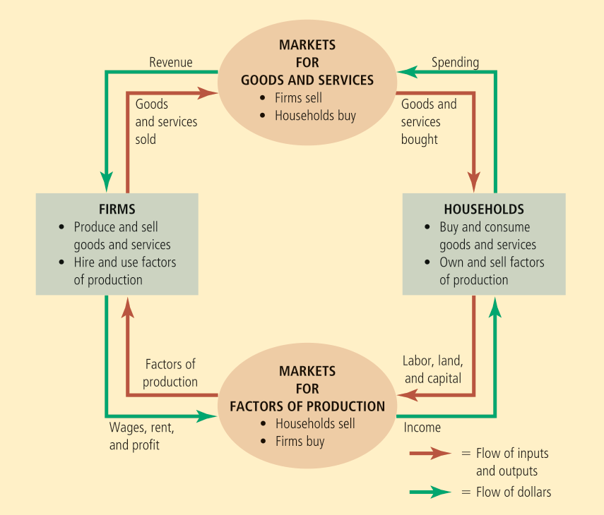
The circular flow diagram doesn’t show everything, factors such as the government and international trade are not considered at all.
The production possibilities frontier is a graph that shows the combinations of output that the economy can produce given the available factors of production and technology.
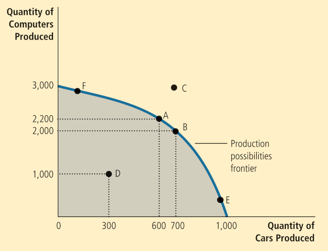
An outcome is efficient if the economy is getting all it can given the constraints. Points on (not inside) the PPF such as A, B, E, F represent efficient outcomes. Note that the PPF shows one of the trade-offs we may face. It also shows the opportunity cost of one good measured in terms of another good.
Further note that if we are at say, F, then the workers who are skilled in car-related areas are also working on computers. The PPF usually has this shape and is steeper towards the middle. If the technology for something becomes better, then the PPF will expand along the corresponding axis.
Obviously, it is extremely difficult to get the exact PPF. It is the duty of the government to introduce suitable taxes/subsidies to ensure that the outcome is efficient.
Lecture 3
Microeconomics focuses on the individual parts of the economy and how households/firms make decisions and interact in specific markets, whereas macroeconomics looks at the economy as a whole, looking at economy-wide phenomena such as inflation, unemployment, and economic growth.
Since macroeconomics is essentially made up of a large number of microeconomic systems, it is impossible to understand the former without the latter.
Positive statements are descriptive and attempt to describe the world as it is, whereas normative statements are prescriptive and are statements about how the world should be.
The validity of positive statements can be decided by observing the facts already present, whereas the validity of normative statements are far more subjective in nature.
Economists may disagree about the validity of different positive theories on how the world works. They may also have different ideals and thus different normative views.
A market is a group of buyers and sellers of a particular good/service.
A competitive market is one where are there are many buyers and sellers so that each has a negligible impact on the market price. A seller has little reason to sell at a lower price than the market price and he cannot sell at a higher price because then, buyers will go elsewhere. In perfectly competitive markets (all the goods are the same and no individual buyer/seller can influence the market), buyers and sellers are said to be price takers.
A monopoly on the other end of the spectrum comprises a single seller who sets the price.
An oligopoly means there are not many sellers and the competition is not very aggressive. For example, the telecom market.
Monopolistic competition (monopoly + competition) has many sellers and slightly differentiated products. Each seller may set the price for their own product. For example, the hotel market.
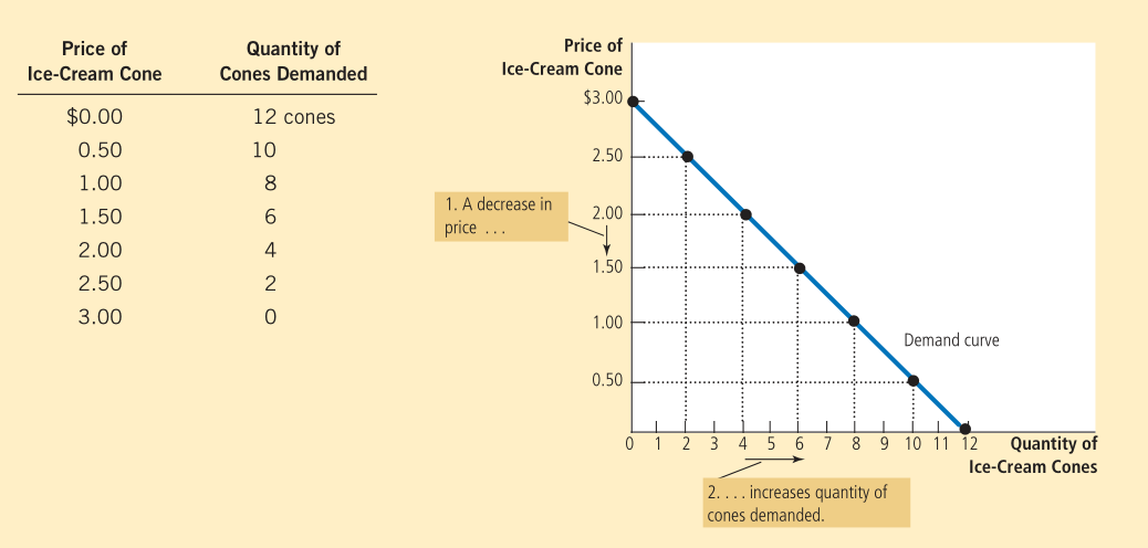
The quantity demanded is the amount of a good that buyers are willing and able to purchase.
The law of demand states that, other things equal, the quantity demanded of a good falls when the price of the good rises.
The law of demand doesn’t always hold. For example, in the stock market, the usual rule of thumb is to buy more when the price of the stocks increases. Another example is paintings/antiques in auctions.
The demand schedule is a table showing the relation between the price and the quantity demanded. When the law of demand holds, the two have an inverse relationship.
The demand curve is a graph of the two (with the price on vertical axis and the quantity demanded on the horizontal).
The following is an example of a demand schedule and curve (following the law of demand).
Lecture 4
The market demand refers to the sum of all the individual demands for a particular good. The market demand curve can be obtained by horizontally summing the individual demand curves.
If a change in some factor shifts the demand curve to the right, it corresponds to an increase in demand (and a shift to the left corresponds to a decrease in demand). Recall that we said “other things constant” while stating the law of demand. What are these other things?
- Income - A normal good is a good for which the demand increases as consumer income increases. A good for which demand falls as income rises is called an inferior good.
- Prices of related goods - When a fall in the price of one good reduces the demand for another good, they are called substitutes. When a fall in the price of one good increases the demand of another, they are called complements.
- Tastes - If general tastes become more tailored towards the product, then demand increases. We don’t often try to explain tastes since they are heavily influenced by factors psychological in nature.
- Expectations - If expectations for the future increase, then demand increases, even if there is no logical reason for the rise of expectation in the first place (self-fulfilling expectations). For example, if we expect an increase in our income, we might save less now and spend more.
- Number of buyers - As the number of buyers increases, the demand increases.
It is important to note that changing the price of some good does not result in a shift of the curve, it merely means that we are moving along the curve.
Similar to the definitions for demand, we have various parameters related to supply - quantity supplied, the law of supply, supply schedule, supply curve, and market supply. The law of supply states that other things constant, the quantity supplied of a good rises when its price rises.
Lecture 5
If a change in some factor shifts the supply curve to the right, it corresponds to an increase in supply (and a shift to the left corresponds to a decrease in supply). What are the factors that can cause a shift in the curve?
- Input Prices - If the prices of goods that serve as input (say sugar for ice-cream) in making the good increase, the curve shifts to the left.
- Technology - If the technology advances, the curve shifts to the right.
- Expectations - If the price of some good is expected (by the firm) to increase in the future, the curve shifts to the left because they start hoarding the product. This assumes the good is durable. If it is perishable, we need to sell it by the expiry date anyway.
- Number of sellers - If the number of sellers increases, the curve shifts to the right.
It should be noted that the supply (demand) curve does not take demand (supply) into consideration explicitly.
Equilibrium is the situation where the quantity supplied is equal to the quantity demanded. The equilibrium price and equilibrium quantity are the corresponding price and quantity. This is just the point of intersection of the supply and demand curves. The equilibrium price is also known as the “market-clearing price”.
If the price is higher than the equilibrium price, then the supply is high and the demand is low. This is known as an excess-supply situation. The excess supply is known as a surplus. Since the sellers need to clear their excess, the price decreases until the equilibrium is reached.
Similarly, if the price is lower than the equilibrium price, we are in an excess-demand situation. The excess demand is known as a shortage. Here, the sellers realize that they need to sell more and they drive up the price until the equilibrium is reached.
Therefore, regardless of how the original situation is, we converge to the equilibrium assuming there are no barriers to this. This phenomenon is known as the law of supply and demand - the price of any good adjusts to bring the quantity supplied and demanded into balance.
Note that this phenomenon is just Adam Smith’s “invisible hand” mentioned in the first lecture and the price system is how it influences the economy.
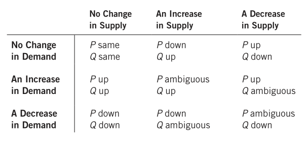
The earlier discussion about shifts of the supply and demand curves can now be used to analyze the shift in equilibria as well. The following table describes how it changes with shift in the curves.
As an aside, it is worth noting that in digital markets, since information transfer is very fast, it doesn’t take too long to attain the new equilibrium if the equilibrium shifts.
Lecture 6
If we map the demand/supply curve with the price on the X-axis instead of the Y-axis, it is sometimes known as the inverse demand/supply curve.
The price elasticity of supply measures how much the quantity supplied changes with the price. If the supply changes substantially with a change in price, it is said to be elastic. If not, it is called inelastic.
A perfectly inelastic supply is one where the quantity supplied does not depend on the price at all. An example of this is beach-front land - irrespective of the price, there is a constant total amount.
Lecture 7
Similar to the price elasticity of supply, we define the price elasticity of demand. There are several factors that must be taken into account when analyzing it:
- Availability of substitutes - Goods with close substitutes tend to have higher elasticity because consumers can easily switch between goods.
- Necessities v. luxuries - Necessities usually have inelastic demands whereas luxuries have elastic demands. Whether something is a necessity or a luxury depends on the properties of the buyer, it is not some intrinsic property of the good.
- Definition of the market - By “definition”, we mean where we draw the boundaries of the market. Narrowly defined markets such as that of vanilla ice-cream are very elastic whereas broadly defined markets such as that of food are inelastic.
- Time horizon - If we have a longer time to adjust, the demand tends to be more elastic.
How do we calculate the price elasticity of demand/supply? We divide the percentage change in the demand/supply by the percentage change in the price. To bring about symmetry, we take the percentage change about the midpoint. So for demand, the price elasticity between two points \((P_1,Q_1)\) and \((P_2,Q_2)\) is
\[\frac{(Q_2-Q_1)/((Q_1+Q_2)/2)}{(P_2-P_1)/((P_1+P_2)/2)}.\]The price elasticity of supply can be calculated similarly.
The demand is said to be
- perfectly inelastic if the price elasticity is equal to \(0\),
- inelastic if the price elasticity is between \(0\) and \(1\),
- unitary if the price elasticity is equal to \(1\),
- elastic if the price elasticity is greater than \(1\), and
- perfectly elastic if the price elasticity is infinite (the demand curve is horizontal).
The total revenue is equal to the price of the good multiplied by the quantity of the good sold.
The change of the total revenue with price depends on the price elasticity.
Note that in a perfectly inelastic situation, reducing the price results in the total revenue decreasing proportionately.
- If the demand is inelastic, total revenue and price grow together.
- If the demand is elastic, total revenue and price grow against each other.
- If the demand is unitary, the total revenue does not change with price.
If the demand decreases linearly with price, then it goes from elastic to unitary to inelastic as demand increases.
The income elasticity of demand measures how much the quantity demanded changes with the income of the consumer. Similar to before, it is calculated by dividing the percentage changes in each. Income elasticity is positive for normal goods and negative for inferior goods.
Lecture 8
The cross-price elasticity of demand measures how the quantity demanded of one good responds to a change in the price of another good. It can be calculated by dividing the percentage change in quantity demanded of the first good by the percentage change in the price of the other good.
Substitutes have positive cross-price elasticity and complements have negative cross-price elasticity.
Until now, we haven’t involved the government at all. In a free, unregulated system, the market forces establish equilibria. While they may be efficient, it needn’t be true that everyone is satisfied in this case. It is the economists’ duty to use theories to assist the development of policies.
Price control is enacted only when these policy-makers believe that the market price is unfair to either the buyers or the sellers. This results in price ceilings (legal maximum price) and floors (legal minimum price).
The price ceiling is said to be binding if it is set below the equilibrium price and not binding if it is set above the equilibrium price. In a competitive market, a binding ceiling results in a shortage and the sellers must ration the scarce goods among the large number of potential buyers.
For example, rent control policy helps the poor by making pricing more affordable (for the poor).
It is worth noting that rent control is usually considered terrible by economists (despite it sounding good to the general public). As with any binding price ceiling, rent control results in a shortage in the long run. On the supply side, landlords are unmotivated to build new apartments and do not maintain the existing ones. On the demand side, people are encouraged to go out and find a place to live. Further, since there is no incentive for landlords to respond to their tenants’ demands, the quality of housing goes down as well. This problem does not show itself in the short run.
An example of a price floor is the minimum wage that is usually present. Similar to rent control, this causes unemployment in the long run. This might be the only reason unpaid internships even exist; inexperienced people (teenagers) are willing to work for nothing (since this circumvents minimum wage).
Lecture 9
Governments levy taxes to raise revenue for public projects. Taxes discourage market activity. When a good is taxed, the quantity sold is reduced.
However, the question is: when a tax is levied, who bears the burden of the tax?
Tax incidence studies this. A tax on the sellers shifts the supply curve (to the left) and a tax on the buyers shifts the demand curve (to the left). In the longer run, taxing the sellers results in the price of the good increasing and taxing the buyers results in the price of the good decreasing (but the price of the good plus the tax increases). This allows us to analyze how the equilibrium changes.
It should be noted that regardless, buyers end up paying more and sellers receive less. So no matter how the tax is levied, the buyers and sellers share the burden, either directly or indirectly. The two taxes are equivalent!
For a payroll tax, the difference between the wage the firm pays and what the worker receives is called the tax wedge, which is just the volume of the tax that goes to the government.
The burden usually ends up being heavier on the side of the market that is less elastic. Indeed, a small elasticity means that the people don’t really have any alternatives, so they stick with the good even if it is actually a bad.
So for a payroll tax, the workers bear most of the burden, not the firms.
Lecture 10
Typically, the goal of the firm is to maximize profits. Sometimes, it may not be - consider the Indian railways. It may also be the goal to maximize sales (equivalently, revenue).
The total revenue is the amount a firm receives for the sale of its output.
The total cost is the market value of the inputs the firm uses in production.
The profit is the total revenue minus the total cost.
Explicit costs are costs that require money, whereas implicit costs are costs that do not (such as opportunity costs). As a result, the accounting profit is quite different from the economic profit (since we include opportunity costs in the latter).
When the total revenue exceeds both explicit and implicit costs, the firm earns economic profit. The economic profit is lower than the accounting profit due to the extra opportunity costs incurred.
The relationship between quantity of input and quantity of output is called the production function.
The marginal product of any input in the production process is the increase in output obtained from one additional unit of input. As input increases, the marginal product decreases - this property is known as diminishing marginal product. This phenomenon is similar to the idiom “Too many cooks spoil the broth”. As marginal product declines, the production function grows flatter.
Fixed costs do not vary with the quantity of output (for example, office space rent) whereas variable costs depend on the quantity of output (for example, the total salaries of workers). The total cost is equal to the sum of the two.
The average total cost is the total cost divided by the quantity of output \(\text{TC}/\text{Q}\). Similarly, we can define average fixed cost and average variable cost.
The marginal cost is the amount the cost increases on increasing production by one unit of output. It is equal to the slope of the total cost function \(\Delta\text{TC}/\Delta\text{Q}\). It is equal to the slope of the total cost function (if it is a continuous cost).
Marginal cost eventually increases with the amount of output produced - this reflects the concept of diminishing marginal product.
The average total cost curve is U-shaped. This is because the average fixed cost decreases whereas the average variable cost increases due to diminishing marginal product.
The average total cost rises (falls) when the marginal cost is greater (less) than than the average total cost.
The marginal cost curve crosses the average total cost curve at the efficient scale. This is the minimum of the average total cost.
Lecture 11
In the short run, some costs are fixed. In the long run, all fixed costs become variable costs.
As a result, a firm’s long-run cost curves differ from its short-run cost curves. The lower envelope of the short-run total average cost curve forms the long-run total average cost curve.
Economies of scale refer to the property whereby long-run average total cost falls as the quantity of output increases.
Diseconomies of scale refer to the property whereby long-run average total cost rises as the quantity of output increases.
Constant economies of scale refer to the property whereby long-run average total cost stays constant as the quantity of output increases.
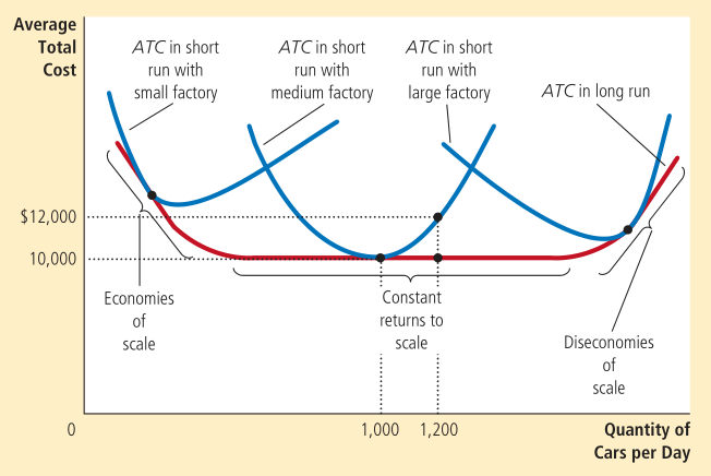
Economies of scale usually occur due to the workers specializing in particular areas. Diseconomies of scale on the other hand might occur due to coordination problems.
In a competitive market,
- There are many buyers and sellers
- The goods offered by the various sellers are largely the same
Each buyer and seller is a price taker. They must accept the price determined by the market.
In a perfectly competitive market, in addition to the above two conditions, firms can freely enter/exit the market.
So, the actions of any single buyer/seller have negligible impact on the market price. The average revenue for any firm is equal to the price of the good. The marginal revenue is also equal to the price of the good and the total revenue is proportional to the quantity of output.
Any firm decides to increase/decrease its output depending on whether the marginal revenue is greater/less than the marginal cost. Because the firm’s marginal cost curve determines the quantity of good the firm is willing to supply at any price, the marginal cost curve is equal to the supply curve.
In the short run, it is difficult to leave the market whereas it is easy in the long run.
A shutdown refers to a short run decision to not produce anything in some period of time due to market conditions. In the short run, the fixed costs cannot be avoided so they continue to be incurred even if a shutdown occurs. This fixed cost is said to be a sunk cost.
Exit refers to a long run decision to leave the market. After a firm exits the market, it incurs neither fixed nor variable costs.
The firm shuts down if the revenue it would earn from producing is less than the variable costs of production. Alternatively, it shuts down if the price is less than the average variable cost.
The firm decides to exit if the revenue is less than the total cost or alternatively, the price is less than the average total cost.
Therefore, the firm’s short run supply curve is that portion of the marginal cost curve which is above the average variable cost curve.
The long run supply curve has the portion of the marginal cost curve which is above the average total cost curve.
Lecture 12
In the long run, the price becomes equal to the minimum of the average total cost (across firms).
As a result, at the end, firms that remain in the market must be making zero economic profit. Firms stop entering/exiting the market only when price and the average total cost are forced to become equal. They are then operating at efficient scale.
This makes sense because the opportunity costs which are taken into account cover other things. The economic profit is zero, not the accounting profit!
In the short run, an increase in demand raises price and quantity supplied (and they make positive economic profit). The resulting influx of firms would force the cost back down, which again results in the long run average total cost being stationary.
While a competitive firm is a price taker, a monopoly firm is a price maker.
A firm is considered a monopoly if it is the sole seller of its product and its product does not have any close substitutes. Monopolies arise when there is a barrier to entry such as
- Ownership of a key resource.
- Government regulation - the government gives a single firm the exclusive right to produce some good.
- The production process - A single firm can supply a good or service to an entire market at a smaller cost than could two or more firms. Costs of production make a single producer more efficient than a large number of producers. In this case, the industry is said to be a natural monopoly. Consider the railways in India.
Lecture 13
If a firm has the first mover’s advantage, they have a good chance of naturally establishing a monopoly. It becomes quite difficult for new people to enter the market.
Because a monopoly has market power, price would rise if they decide to produce less (as opposed to a competitive market where the price remains constant irrespective of quantity produced). The demand curve is downwards sloping.
A monopoly’s marginal revenue is always less than the price (so the marginal revenue curve is always below the demand/average revenue curve). This is because if it wants to sell more units, it should reduce the price it charges to the customers.
When the quantity supplied by a monopoly increases, the quantity sold increases (output effect) but the price falls as well (price effect).
Profit is maximized when the marginal cost is equal to the marginal revenue. At this point, for a monopolistic firm, the price exceeds the marginal cost.
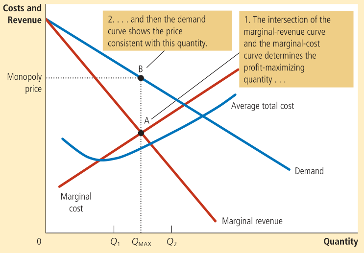
Remember that all profit-maximizing curves try to equalize the marginal revenue and marginal cost. The monopoly profits as long as the price is greater than the average total cost.
Price discrimination is the practice of selling the same good at different prices to different customers, even though the costs of production are the same.
To price discriminate, the firm must have market power. In perfect price discrimination, the monopolist knows the willingness to pay of each customer and charges each customer a different price.
It is not possible in a competitive market since the seller requires market power to enforce it.
Price discrimination increases profits for the monopolist.
Welfare economics studies how the allocation of resources affects economic wellbeing.
Equilibrium in the market ensures maximum welfare for both the consumers and the producer.
The willingness to pay is the maximum amount that a buyer will pay for a good. The consumer surplus is the buyer’s willingness to pay for a good minus the amount they actually pay for it. The area below the demand curve and above the price measures the consumer surplus.
Lecture 14
Consumer surplus measures the benefit the buyer receives from a good as they perceive it.
Producer surplus is the amount a seller is paid for a good minus the cost. Just like before, the area above the supply curve and below the price measures the producer surplus.
The total surplus is the sum of the consumer surplus and producer surplus. A resource allocation is said to exhibit efficiency if it maximizes total surplus. Equality (or equity) checks whether the producers and consumers have similar levels of economic wellbeing.
- Free markets allocate the supply to buyers who value them most (as measured by their willingness to pay).
- Free markets allocate the demand to sellers who can produce them at the lowest cost.
- Free markets produce the quantity of goods that maximizes the sum of consumer and producer surplus.
Therefore, a social planner should leave a free market alone. This is referred to as laissez faire - letting people do as they will.
This is not the case when there is a market failure due to externalities or market power.
The resulting inefficiency shows itself as deadweight loss, which is equal to the corresponding fall in total surplus.
Imposing a tax can manifest in a deadweight loss.
When buyers/sellers do not take externalities into account, the equilibrium could be inefficient.
The theory of consumer choice asks
- whether all demand curves slope downward,
- how wages affect labor supply, and
- how interest rates affect household saving.
Budget constraint depicts the limit on the consumption bundles that a consumer can afford.
It limits the various combinations of goods that the consumer can afford given their income and the prices. A budget constraint curve looks like:
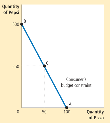
The slope of the curve is equal to the ratio of the two prices, the relative price.
We should also take preferences into account. For this, we draw the indifference curve.
An indifference curve shows consumption bundles that give the consumer the same level of satisfaction. The slope at any point represents how much of one good the consumer is willing to give up for one unit of the other - this is known as the marginal rate of substitution.
The slope at any point on an indifference curve is the marginal rate of substitution. It represents how much of one good the consumer is willing to give up for one unit of the other.
Lecture 15
- Higher indifference curves are preferred to lower ones - consumers prefer to have more of something.
- Indifference curves are downward sloping - consumers are willing to give up some good only if they get some other good in return.
- Indifference curves do not cross.
- Indifference curves are bowed inwards - consumers are more willing to trade away goods they have in abundance.
Perfect substitutes are goods with straight-line indifference curves. As a result, the marginal rate of substitution is constant. For example, nickels and dimes.
Goods with right-angle indifference curves are perfect complements. For example, left shoes and right shoes.
A point at which the budget constraint curve and an indifference curve touch (tangentially) is known as the optimum.
Therefore, the consumer chooses to consume such that the marginal rate of substitution is equal to the relative price. We are just equating the slope of the indifference curve and the slope of the budget constraint. At the optimum, the valuation of the two goods equals the market’s valuation.
An increase in income shifts the budget constraint curve outwards.
The substitution effect is the change in consumption that occurs when a price change moves the consumer along an indifference curve to a point with a different marginal rate of substitution (along the indifference curve).
The income effect is the change in consumption that occurs when a price change moves the consumer to a higher or lower indifference curve.
Lecture 16
A fall in the price of some good rotates the budget constraint curve. This changes the slope as well. It pivots around the point of intersection corresponding to the price that has not changed.
The change due to the income and substitution effects can be thought to occur in two parts.
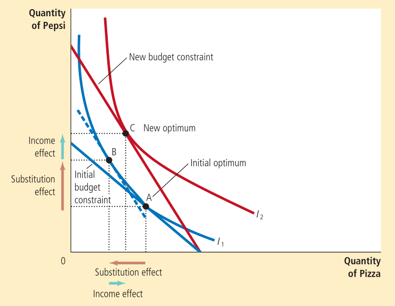
The change from A to B is the substitution effect, where we move along the same indifference curve. The change from B to C is the income effect, where the two points have the same marginal rate of substitution. C is the optimum for the corresponding indifference curve.
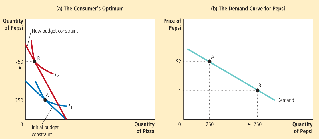
Now, we can derive the demand curve of the consumer using the budget constraint and indifference curves. This can be understood using the following example.
It is also possible for the demand curve to slope upwards if the income effect strongly dominates the substitution effect for an inferior good. Such a good that violates the law of demand is known as a Giffen good. As the cost increases, the quantity demanded increases as well.
For a normal good, the income effect results in an increase in consumption whereas for an inferior good, it results in a decrease in consumption. Therefore, for normal goods, both the effects work in the same direction and the consumption increases when price increases. For an inferior good, they work in opposite directions.
Lecture 17
Suppose we have two goods consumption and leisure. Suppose the wage goes up and the cost of the first increases, the substitution effect says that the consumption of the latter should decrease. On the other hand, the income effect says that the consumption of the latter should increase since we have more disposable income now.
If the substitution effect is greater than the income effect, they reduce leisure and work more. We must determine which dominates to analyze the situation.